| size | prob |
|---|---|
| 1 | 0.267 |
| 2 | 0.336 |
| 3 | 0.158 |
| 4 | 0.137 |
| 5 | 0.063 |
| 6 | 0.024 |
| 7 | 0.015 |
5 Discrete Probability Distribution
When computing probabilities, the sample space, which contains all the outcomes of the experiment, is listed. If the probabilities for all of the outcomes are also listed then these two together are called a probability distribution. With a probability distribution, the shape can be determined, the mean and standard deviation can be calculated, and the probability of events can be found. How to find all of these concepts depends on what type of quantitative variables are being considered. Remember there are different types of quantitative variables, called discrete or continuous. What is the difference between discrete and continuous data? Discrete data can only take on particular values in a range. Continuous data can take on any value in a range. Discrete data usually arises from counting while continuous data usually arises from measuring.
If you have a variable, and can find a probability associated with that variable, it is called a random variable. In many cases the random variable is what you are measuring, but when it comes to discrete random variables, it is usually what you are counting. So for the example of how tall is a plant given a new fertilizer, the random variable is the height of the plant given a new fertilizer. For the example of how many fleas are on prairie dogs in a colony, the random variable is the number of fleas on a prairie dog in a colony.
5.0.1 Examples of each:
How tall is a plant given a new fertilizer? Continuous. This is something you measure.
How many fleas are on prairie dogs in a colony? Discrete. This is something you count.
Now suppose you put all the values of the random variable together with the probability that the random variable would occur. You could then have a distribution like before, but now it is called a probability distribution since it involves probabilities. A probability distribution is an assignment of probabilities to the values of the random variable.
With the idea of a probability distribution, the next thing is to look at the basics of a probability distribution.
5.1 Basics of Probability Distributions
As a reminder, a variable or what will be called the random variable from now on, is represented by the letter \(x\) and it represents a quantitative (numerical) variable that is measured or observed in an experiment.
As with probabilities, probability distributions, have the properties, \(0 \le P(outcome)\le1\) and \(\sum{P(outcomes)}=1\)
5.1.1 Example: Probability Distribution
The 2010 U.S. Census found the chance of a household being a certain size. The data is in Table 5.1 (\“Households by age,\” 2013). Note, the category 7 is really 7 or more people in the household. Draw the probability distribution and find the mean, variance, and standard deviation.
5.1.1.1 Solution
In this case, the random variable is \(x\) = size of household. This is a discrete random variable, since you are counting the number of people in a household.
It is a probability distribution since you have the \(x\) value and the probabilities that go with it, all of the probabilities are between zero and one, and the sum of all of the probabilities is one.
You can give a probability distribution in table form (as in Table 5.1) or as a graph. The graph looks like a histogram. To graph the histogram, use the following commands and process in rStudio.
First you need to load a few packages using the following commands. These packages are “arm” and “Weighted.Desc.Stat”. If these packages have not been installed, they need to be installed before you can load them using library. Once you have installed them, they will always be available in /r Studio to be loaded. To load a package, use the command
library(“name of package”)
In this case the packages you need are arm and Weighted.Desc.Stat.
Loading required package: MASSLoading required package: MatrixLoading required package: lme4
arm (Version 1.13-1, built: 2022-8-25)Working directory is /Users/kathrynkozak/Statistics_book/Statistics-Using-Technology-bookTo draw the probability distribution, use the following command. First you need to create variables for \(x\), size, and the probability, \(prob\), in r Studio. Then you can draw the distribution.
(ref:discrete-histogram-cap) Histogram of Size of Family
discrete.histogram(Household$size,Household$prob, bar.width = 1, main="Size of family", xlab="Size") 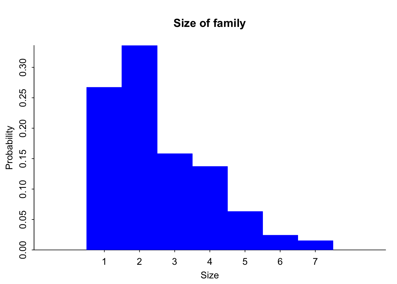
This command is different than the commands used in the past, but is needed for discrete probability distributions. So putting a title on the graph uses the command main=“title you want” instead of title= as before.
Notice this graph Figure 5.1 is skewed right, which means that most families have around 2 people in them and larger families become more and more rare.
To find the mean, variance, and standard deviation using r Studio, make sure that the package Weighted.Desc.Stat is loaded, then use the following commands.
w.mean(Household$size, Household$prob) [1] 2.525w.var(Household$size, Household$prob) [1] 2.023375w.sd(Household$size, Household$prob)[1] 1.422454The mean is 2.525 people, the variance is 2.02 \(people^2\), and the standard deviation is 1.42 people.
When calculating the mean and standard deviation of a probability distribution, you can consider the population distribution the population even though it was most likely created from a large sample. Since a probability distribution is basically a population, the mean and standard deviation that are calculated are actually the population parameters and not the sample statistics. The notation used is the same as the notation for population mean, \(\mu\), and population standard deviation, $\sigma$, that was used in chapter 3. Note: the mean can also be thought of as the expected value. It is the value you expect to get if the trials were repeated infinite number of times. The mean or expected value does not need to be a whole number, even if the possible values of \(x\) are whole numbers. This means one can find what value they can expect to get in the long run for gambling or insurance including extended warranties using the mean of a probability distribution. First one needs to figure out the probability distribution, and then follow the process in example 5.1.1.
5.1.2 Example: Calculating the Expected Value
In the Arizona lottery game called Pick 3, a player pays \$1 and then picks a three-digit number. If those three numbers are picked in that specific order the person wins \$500. What is the expected value in this game?
5.1.2.1 Solution
To find the expected value, you need to first create the probability distribution. In this case, the random variable \(x\) = winnings. If you pick the right numbers in the right order, then you win \$500, but you paid \$1 to play, so you actually win \$499. If you didn’t pick the right numbers, you lose the \$1, the \(x\) value is $-1$. You also need the probability of winning and losing. Since you are picking a three-digit number, and for each digit there are 10 numbers you can pick with each independent of the others, you can use the multiplication rule. To win, you have to pick the right numbers in the right order. The first digit, you pick 1 number out of 10, the second digit you pick 1 number out of 10, and the third digit you pick 1 number out of 10. The probability of picking the right number in the right order is $\frac{1}{1000}$. The probability of losing (not winning) would be
\(1-\frac{1}{1000}=\frac{999}{1000}\).
Putting this information into a table will help to organize the information and find the expected value.
| outcome | amount | probability |
|---|---|---|
| win | 499 | 0.001 |
| lose | -1 | 0.999 |
Now type the values into r using the following command:
Now to find the expected value, it is the same as finding the mean, though the command is a little different since you don’t have a data frame for this data.
weighted.mean(amount, probability)[1] -0.5The expected value (or mean) is -0.5. That is -\$0.50. Since it is negative, that means you lose \$0.50 every time you play the Pick 3. It seems you would be better off putting the \$1 every week into a savings account then playing the Pick 3 lottery.
The reason probability is studied in statistics is to help in making decisions in inferential statistics. To understand how that is done the concept of a rare event is needed.
5.1.3 Rare Event Rule for Inferential Statistics
If, under a given assumption, the probability of a particular observed event is extremely small, then you can conclude that the assumption is probably not correct.
An example of this is suppose you roll an assumed fair die 1000 times and get a six 600 times, when you should have only rolled a six around 160 times, then you should believe that your assumption about it being a fair die is untrue.
5.1.4 Determining if an event is unusual
If you are looking at a value of \(x\) for a discrete variable, and the P(the variable has a value of \(x\) or more) is less than 0.05, then you can consider the \(x\) an unusually high value. Another way to think of this is if the probability of getting such a high value is less than 0.05, then the event of getting the value x is unusual.
Similarly, if the P(the variable has a value of \(x\) or less) is less than 0.05, then you can consider this an unusually low value. Another way to think of this is if the probability of getting a value as small as \(x\) is less than 0.05, then the event \(x\) is considered unusual.
Why is it “\(x\) or more” or “\(x\) or less” instead of just “\(x\)” when you are determining if an event is unusual? Consider this example: you and your friend go out to lunch every day. Instead of Going Dutch (each paying for their own lunch), you decide to flip a coin, and the loser pays for both. Your friend seems to be winning more often than you’d expect, so you want to determine if this is unusual before you decide to change how you pay for lunch (or accuse your friend of cheating). The process for how to calculate these probabilities will be presented in the next section on the binomial distribution. If your friend won 6 out of 10 lunches, the probability of that happening turns out to be about 20.5%, not unusual. The probability of winning 6 or more is about 37.7%. But what happens if your friend won 501 out of 1,000 lunches? That doesn’t seem so unlikely! The probability of winning 501 or more lunches is about 47.8%, and that is consistent with your hunch that this isn’t so unusual. But the probability of winning exactly 501 lunches is much less, only about 2.5%. That is why the probability of getting exactly that value is not the right question to ask: you should ask the probability of getting that value or more (or that value or less on the other side).
The value 0.05 will be explained later, and it is not the only value you can use for unusual events.
5.1.5 Example: Is the Event Unusual
The 2010 U.S. Census found the chance of a household being a certain size. The data is in the table (\“Households by age,\” 2013).
The 2010 U.S. Census found the chance of a household being a certain size. The data is in Table 5.1 (\“Households by age,\” 2013). Note, the category 7 is really 7 or more people in the household.
State random variable:
Solution
State random variable
- Is it unusual for a household to have six people in the family?
size = number of people in a household
- Is it unusual for a household to have six people in the family?
- If you did come upon many families that had six people in the family, what would you think?
- Is it unusual for a household to have four people in the family?
- If you did come upon a family that has four people in it, what would you think?
5.1.5.1 Solution
To determine this, you need to look at probabilities. However, you cannot just look at the probability of six people. You need to look at the probability of \(x\) being six or less people or the probability of \(x\) being six or more people. The
\(P(x \le 6)=P(1)+P(2)+P(3)+P(4)+P(5)+P(6)\) \(=0.267+0.336+0.158+0.137+0.063+0.024=0.985\)
Since this probability is more than 5%, then six is not an unusually low value.
The \(P(x \ge 6)=P(6)+P(7)=0.024+0.015=0.039\)
Since this probability is less than 5%, then six is an unusually high value. It is unusual for a household to have six people in the family.
- If you did come upon many families that had six people in the family, what would you think?
Since it is unusual for a family to have six people in it, then you may think that either the size of families is increasing from what it was or that you are in a location where families are larger than in other locations.
- Is it unusual for a household to have four people in the family?
To determine this, you need to look at probabilities. Again, look at the probability of \(x\) being four or less or the probability of \(x\) being four or more. The
\(P(x \le 4)=P(0)+P(1)+P(2)+P(3)+P(4)\) \(=0.267+0.336+0.158+0.137=0.898\)
Since this probability is more than 5%, four is not an unusually low value.
The
\(P(\ge4)=P(4)+P(5)+P(5)+P(7)\) \(=0.137+0.063+0.024+0.015=0.239\)
Since this probability is more than 5%, four is not an unusually low value. Thus, four is not an unusual size of a family.
- If you did come upon a family that has four people in it, what would you think?
Since it is not unusual for a family to have four members, then you would not think anything is amiss.
5.1.6 Homework for Basics of Probability Distributions Section
- Eyeglassomatic manufactures eyeglasses for different retailers. The number of days it takes to fix defects in an eyeglass and the probability that it will take that number of days are in Table 5.2.
Days<- read.csv(
  "https://krkozak.github.io/MAT160/table_5_1_3.csv")
knitr::kable(Days)| days | prob |
|---|---|
| 1 | 0.249 |
| 2 | 0.108 |
| 3 | 0.091 |
| 4 | 0.123 |
| 5 | 0.133 |
| 6 | 0.114 |
| 7 | 0.070 |
| 8 | 0.046 |
| 9 | 0.019 |
| 10 | 0.013 |
| 11 | 0.010 |
| 12 | 0.008 |
| 13 | 0.006 |
| 14 | 0.004 |
| 15 | 0.002 |
| 16 | 0.002 |
| 17 | 0.001 |
| 18 | 0.001 |
- State the random variable.
- Draw a histogram of the number of days to fix defects
- Find the mean number of days to fix defects.
- Find the variance for the number of days to fix defects.
- Find the standard deviation for the number of days to fix defects.
- Find probability that a lens will take at least 16 days to make a fix the defect.
- Is it unusual for a lens to take 16 days to fix a defect?
- If it does take 16 days for eyeglasses to be repaired, what would you think?
- Suppose you have an experiment where you flip a coin three times. You then count the number of heads.
- State the random variable.
- Write the probability distribution for the number of heads.
- Draw a histogram for the number of heads.
- Find the mean number of heads.
- Find the variance for the number of heads.
- Find the standard deviation for the number of heads.
- Find the probability of having two or more number of heads.
- Is it unusual for to flip two heads?
The Ohio lottery has a game called Pick 4 where a player pays \$1 and picks a four-digit number. If the four numbers come up in the order you picked, then you win \$2,500. What is your expected value?
An LG Dishwasher, which costs \$800, has a 20% chance of needing to be replaced in the first 2 years of purchase. A two-year extended warranty costs \$112.10 on a dishwasher. What is the expected value of the extended warranty assuming it is replaced in the first 2 years?
5.2 Binomial Probability Distribution
Section 5.1 introduced the concept of a probability distribution. The focus of the section was on discrete probability distributions. To find the probability distribution for a situation, you usually needed to actually conduct the experiment and collect data. Then you can calculate the experimental probabilities. Normally you cannot calculate the theoretical probabilities. However, there are certain types of experiment that allow you to calculate the theoretical probability. One of those types is called a Binomial Experiment.
Properties of a binomial experiment (or Bernoulli trial):
Fixed number of trials, \(n\), which means that the experiment is repeated a specific number of times.
The \(n\) trials are independent, which means that what happens on one trial does not influence the outcomes of other trials.
There are only two outcomes, which are called a success and a failure.
The probability of a success doesn’t change from trial to trial, where \(p\) = probability of success and \(q = 1-p\) = probability of failure.
If you know you have a binomial experiment, then you can calculate binomial probabilities. This is important because binomial probabilities come up often in real life. Examples of binomial experiments are:
Toss a fair coin ten times, and find the probability of getting two heads.
Question twenty people in class, and look for the probability of more than half being women?
Shoot five arrows at a target, and find the probability of hitting it five times?
5.2.1 Formula for the probabilities for a Binomial experiment
First, the random variable in a binomial experiment is \(x\) = number of successes.
Be careful, a success is not always a good thing. Sometimes a success is something that is bad, like finding a defect. A success just means you observed the outcome you wanted to see happen.
Binomial Formula for the probability of \(r\) successes in \(n\) trials is \(P(X=r)=_nC_r*p^r*q^{n-r}\)
where \(_nC_r\) is the number of combinations of \(n\) things taking \(r\) at a time. It is read “\(n\) choose \(r\)”.
When solving problems, make sure you define your random variable and state what \(n, p\), and \(r\) are. Without doing this, the problems are a great deal harder.
The command to find a binomial probability in r Studio is
P\((X=r)=\)
dbinom(r, n, p)
\(P(x \le r)=\)
pbinom(r, n, p, lower.tail=TRUE)
\(P(x \ge r)=\)
pbinom(r-1, n, p, lower.tail = FALSE)
5.2.2 Example: Calculating Binomial Probabilities
When looking at a person’s eye color, it turns out that 1% of people in the world has green eyes (“What percentage of,” 2013). Consider a group of 20 people.
- State the random variable.
- Argue that this is a binomial experiment
- Find the probability that none of the 20 people have green eyes.
- Find the probability that nine have green eyes.
- Find the probability that at most three have green eyes.
- Find the probability that at most two have green eyes.
- Find the probability that at least four have green eyes.
- In Europe, four people out of twenty have green eyes. Is this unusual? What does that tell you?
5.2.2.1 Solution
- State the random variable.
\(x\) = number of people with green eyes
- Argue that this is a binomial experiment.
There are 20 people, and each person is a trial, so there are a fixed number of trials. In this case, \(n\) = 20.
If you assume that each person in the group is chosen at random the eye color of one person doesn’t affect the eye color of the next person, thus the trials are independent.
Either a person has green eyes or they do not have green eyes, so there are only two outcomes. In this case, the success is a person has green eyes.
The probability of a person having green eyes is 0.01. This is the same for every trial since each person has the same chance of having green eyes.
- Find the probability that none of the 20 people have green eyes.
If none have green eyes, then \(r=0\).
Probability that none have green eyes is \(P(X=0)=0.818\), using the command:
dbinom(0,20,0.01) [1] 0.8179069- Find the probability that nine have green eyes.
If nine have green eyes, then \(r=9\).
Probability that 9 have green eyes is
\(P(X=9)=1.50X10^{-13}\). Notice that r gives the answer as 1.50391e-13. This is the way many computer programs write a number in scientific notation. It isn’t possible for a computer to write it as \(1.50381X10^{-13}\), but it is possible for humans to write it correctly. So make sure the answer is written in the correct scientific notation.
dbinom(9,20,0.01)[1] 1.50381e-13- Find the probability that at most three have green eyes.
At most three means that three is the highest value you will have. Find the probability of \(x\) is less than or equal to three.
Since this is less than, then the lower tail of the probability distribution is being used, so \(P(X \le 3)=0.99996\) using the command in r Studio of
pbinom(3,20,0.01, lower.tail=TRUE)[1] 0.9999574The reason the answer is written to more decimal places is because when it is rounded to three decimal places the rounding makes the answer 1. But 1 means that the event will happen, when in reality there is a slight chance that it won’t happen. It is best to write the answer to more decimal places or it can be written as \(>0.999\) to represent that the number is very close to 1, but isn’t 1.
- Find the probability that at most two have green eyes.
At most 2 means 2 or less. So find the probability that there are less than or equal to 2. \(P(X \le 2)=0.999\), and again, this is the lower tail of the probability distribution, so use lower.tail=TRUE in the r command:
pbinom(2,20,0.01, lower.tail=TRUE)[1] 0.9989964- Find the probability that at least four have green eyes.
At least four means four or more. Find the probability of \(x\) being greater than or equal to four. Since it is greater than or equal to, this is the right tail of the probability distribution. However, if you just use lower.tail=FALSE, then the 4 is not included in r calculations. You want all numbers from 4 on up, so you need to use
\(r=4-1=3\) in the r command. This will include 4 in the calculation. \(P(X \ge 4)=4.26X10^{-5}\)
pbinom(4-1,20,0.01, lower.tail=FALSE) [1] 4.262093e-05- In Europe, four people out of twenty have green eyes. Is this unusual? What does that tell you?
Since the probability of finding four or more people with green eyes is much less than 0.05, it is unusual to find four people out of twenty with green eyes. That should make you wonder if the proportion of people in Europe with green eyes is more than the 1% for the general population. If this is true, then you may want to ask why Europeans have a higher proportion of green-eyed people. That of course could lead to more questions.
5.2.3 Example: Calculating Binomial Probabilities
According to the Center for Disease Control (CDC), about 1 in 88 children in the U.S. have been diagnosed with autism (“CDC-data and statistics,” 2013). Suppose you consider a group of 10 children.
- State the random variable.
- Argue that this is a binomial experiment
- Find the probability that none have autism.
- Find the probability that seven have autism.
- Find the probability that at least five have autism.
- Find the probability that at most two have autism.
- Suppose five children out of ten have autism. Is this unusual? What does that tell you?
5.2.3.1 Solution
- State the random variable.
\(x\) = number of children with autism.
- Argue that this is a binomial experiment
There are 10 children, and each child is a trial, so there are a fixed number of trials. In this case, \(n\) = 10.
If you assume that each child in the group is chosen at random, then whether a child has autism does not affect the chance that the next child has autism. Thus the trials are independent.
Either a child has autism or they do not have autism, so there are two outcomes. In this case, the success is a child has autism.
The probability of a child having autism is \(\frac{1}{88}\). This is the same for every trial since each child has the same chance of having autism.
- Find the probability that none have autism.
\(P(X=0)=0.892\)
dbinom(0,10, 1/88)[1] 0.892002- Find the probability that seven have autism.
\(P(X=7)=2.84X10^{-12}\)
dbinom(7,10, 1/88)[1] 2.837346e-12- Find the probability that at least five have autism.
\(P(X \ge 5)=4.553X10^{-8}\). Again, this is the upper tail of the probability distribution, so use lower=tail=FALSE and
\(r=5-1=4\) to make sure that r calculates for 5 and on up.
pbinom(5-1, 10, 1/88, lower.tail=FALSE)[1] 4.553416e-08- Find the probability that at most two have autism.
\(P(X \le 2)=0.9998\). This is using the lower tail of the probability distribution.
pbinom(2, 10, 1/88, lower.tail=TRUE)[1] 0.9998341- Suppose five children out of ten have autism. Is this unusual? What does that tell you?
Since the probability of five or more children in a group of ten having autism is much less than 5%, it is unusual to happen. If this does happen, then one may think that the proportion of children diagnosed with autism is actually more than \(\frac{1}{88}\).
5.2.4 Homework for Binomial Probability Distribution Section
- Approximately 10% of all people are left-handed (\“11 little-known facts,\” 2013). Consider a grouping of fifteen people.
- State the random variable.
- Argue that this is a binomial experiment
- Find the probability that none are left-handed.
- Find the probability that seven are left-handed.
- Find the probability that at least two are left-handed.
- Find the probability that at most three are left-handed.
- Find the probability that at least seven are left-handed.
- Seven of the last 15 U.S. Presidents were left-handed. Is this unusual? What does that tell you?
- According to an article in the American Heart Association’s publication *Circulation*, 24% of patients who had been hospitalized for an acute myocardial infarction did not fill their cardiac medication by the seventh day of being discharged (Ho, Bryson & Rumsfeld, 2009). Suppose there are twelve people who have been hospitalized for an acute myocardial infarction.
- State the random variable.
- Argue that this is a binomial experiment
- Find the probability that all filled their cardiac medication.
- Find the probability that seven did not fill their cardiac medication.
- Find the probability that none filled their cardiac medication.
- Find the probability that at most two did not fill their cardiac medication.
- Find the probability that at least three did not fill their cardiac medication.
- Find the probability that at least ten did not fill their cardiac medication.
- Suppose of the next twelve patients discharged, ten did not fill their cardiac medication, would this be unusual? What does this tell you?
- Eyeglassomatic manufactures eyeglasses for different retailers. In March 2010, they tested to see how many defective lenses they made, and there were 16.9% defective lenses due to scratches. Suppose Eyeglassomatic examined twenty eyeglasses.
- State the random variable.
- Argue that this is a binomial experiment
- Find the probability that none are scratched.
- Find the probability that all are scratched.
- Find the probability that at least three are scratched.
- Find the probability that at most five are scratched.
- Find the probability that at least ten are scratched.
- Is it unusual for ten lenses to be scratched? If it turns out that ten lenses out of twenty are scratched, what might that tell you about the manufacturing process?
- The proportion of brown M&M’s in a milk chocolate packet is approximately 14% (Madison, 2013). Suppose a package of M&M’s typically contains 52 M&M’s.
- State the random variable.
- Argue that this is a binomial experiment
- Find the probability that six M&M’s are brown.
- Find the probability that twenty-five M&M’s are brown.
- Find the probability that all of the M&M’s are brown.
- Would it be unusual for a package to have only brown M&M’s? If this were to happen, what would you think is the reason?
5.3 Mean and Standard Deviation of Binomial Distribution
If you list all possible values of \(x\) in a Binomial distribution, you get the Binomial Probability Distribution. You can draw a histogram of the probability distribution and find the mean (expected value), variance, and standard deviation of it. To have r Studio calculate the binomial values and save them to a variable, use the command
x<-c(0:n) p<-dbinom(0:n, n, p)
5.3.1 Example: Finding the Probability Distribution, Mean, Variance and Standard Deviation of a Binomial Distribution
When looking at a person’s eye color, it turns out that 1% of people in the world has green eyes (“What percentage of,” 2013). Consider a group of 20 people.
- State the random variable.
- Write the probability distribution.
- Draw a histogram.
- Find the mean, variance, and standard deviation.
5.3.1.1 Solution
- State the random variable.
\(x\) = number of people who have green eyes
- Write the probability distribution.
In this case you need to write each value of \(x\) and its corresponding probability. It is easiest to do this by using the r Command:
green<-c(0:20)
probability_green<-dbinom(0:20,20, 0.01)
It looks like nothing happened, but r save the values as variables. To see what is in each of those values, type
green [1] 0 1 2 3 4 5 6 7 8 9 10 11 12 13 14 15 16 17 18 19 20probability_green [1] 8.179069e-01 1.652337e-01 1.585576e-02 9.609552e-04 4.125313e-05
[6] 1.333434e-06 3.367259e-08 6.802543e-10 1.116579e-11 1.503810e-13
[11] 1.670900e-15 1.534344e-17 1.162381e-19 7.225371e-22 3.649177e-24
[16] 1.474415e-26 4.654088e-29 1.106141e-31 1.862190e-34 1.980000e-37
[21] 1.000000e-40These can now be typed into a table if desired.
- Draw a histogram.
On r, this is like what was done in Section 5.1. Makes sure that the packages “arm” and “Weighted.Desc.Stat” are loaded. Then perform the command to get:
discrete.histogram(green, probability_green, bar.width = 1, main="Number of People with Green Eyes", xlab="Numbr of People with Green Eyes")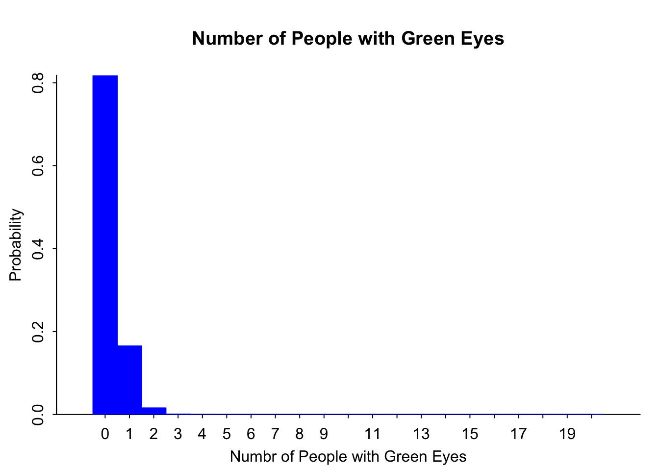
Notice this graph Figure 5.2 is skewed right.
- Find the mean, variance, and standard deviation
Using r Studio command such as those in Section 5.1:
w.mean(green, probability_green) [1] 0.2w.var(green, probability_green) [1] 0.198w.sd(green, probability_green)[1] 0.4449719You expect on average that out of 20 people, less than 1 person would have green eyes, with are variance of 0.198 \(people^2\) and a standard deviation of 0.44 people.
5.3.2 Homework for Mean and Standard Deviation of Binomial Distribution Section
- Suppose a random variable, \(x\), arises from a binomial experiment. Suppose \(n = 6\), and \(p = 0.13\).
- Write the probability distribution.
- Draw a histogram.
- Describe the shape of the histogram.
- Find the mean.
- Find the variance.
- Find the standard deviation.
- Suppose a random variable, \(x\), arises from a binomial experiment. Suppose \(n = 10\), and \(p = 0.81\).
- Write the probability distribution.
- Draw a histogram.
- Describe the shape of the histogram.
- Find the mean.
- Find the variance.
- Find the standard deviation.
- Suppose a random variable, \(x\), arises from a binomial experiment. Suppose \(n = 7\), and \(p = 0.50\).
- Write the probability distribution.
- Draw a histogram.
- Describe the shape of the histogram.
- Find the mean.
- Find the variance.
- Find the standard deviation.
- Approximately 10% of all people are left-handed. Consider a grouping of fifteen people.
- State the random variable.
- Write the probability distribution.
- Draw a histogram.
- Describe the shape of the histogram.
- Find the mean.
- Find the variance.
- Find the standard deviation.
- According to an article in the American Heart Association’s publication *Circulation*, 24% of patients who had been hospitalized for an acute myocardial infarction did not fill their cardiac medication by the seventh day of being discharged (Ho, Bryson & Rumsfeld, 2009). Suppose there are twelve people who have been hospitalized for an acute myocardial infarction.
- State the random variable.
- Write the probability distribution.
- Draw a histogram.
- Describe the shape of the histogram.
- Find the mean.
- Find the variance.
- Find the standard deviation.
- Eyeglassomatic manufactures eyeglasses for different retailers. In March 2010, they tested to see how many defective lenses they made, and there were 16.9% defective lenses due to scratches. Suppose Eyeglassomatic examined twenty eyeglasses.
- State the random variable.
- Write the probability distribution.
- Draw a histogram.
- Describe the shape of the histogram.
- Find the mean.
- Find the variance.
- Find the standard deviation.
- The proportion of brown M&M’s in a milk chocolate packet is approximately 14% (Madison, 2013). Suppose a package of M&M’s typically contains 52 M&M’s.
State the random variable.
Find the mean.
Find the variance.
Find the standard deviation.